
This is part 2 of the 3-part post on Monte Carlo simulations for option selling.
Jump to:
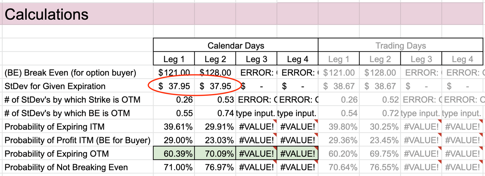
Let’s look at how the simulation results were calculated. By the time we have punched in all the values, the simulation has already run. Scrolling to the right, we see that for each leg of the spread, the standard deviation has been calculated by adjusting the IV to the time period being simulated and converting it into dollars, using the formula below.
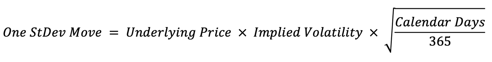
The standard deviation is the same for both legs because it is only based on the current stock price, the implied volatility, and the option term. Note that this calculation is also done using trading days (business days) instead of calendar days, however the rest of the simulation uses the results from the calendar-days calculation. Feel free to experiment with this on your own.
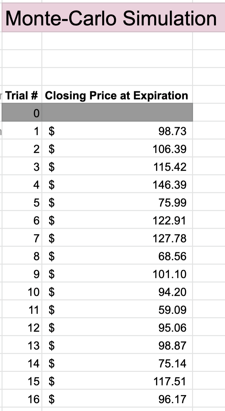
The mean, which is assumed to be the current stock price of $100, and standard deviation are used to generate a normal distribution. One thousand possible closing prices are generated according to this distribution and stored here:
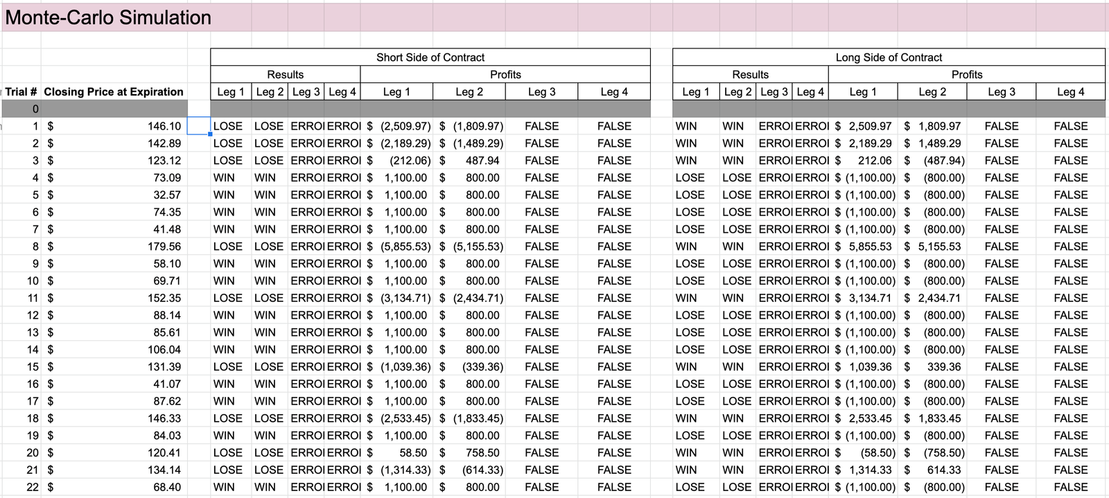
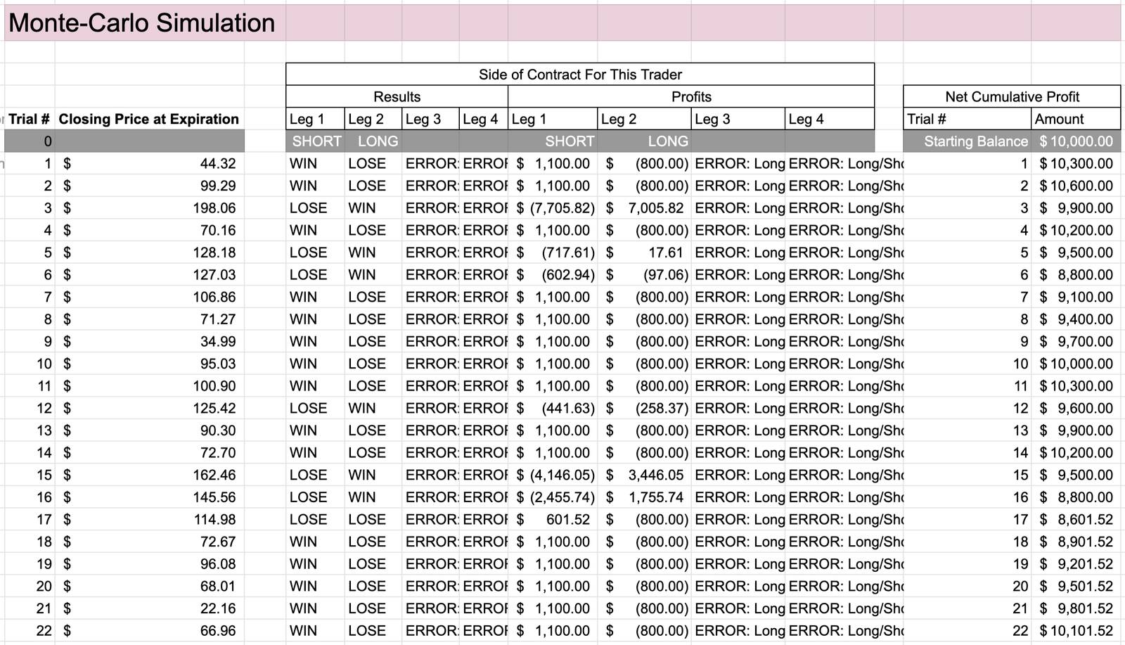
For each simulated closing price, the “WIN” or “LOSE” result and associated profit/loss are calculated for both the short side of the contract and the long side of the contract. This just means that for each leg, your outcome is calculated as if you had sold that option, and as if you had bought that option. The seller’s loss is the buyer’s win, and vice versa.
A “WIN” for the seller is defined as the option expiring OTM, while a “LOSE” is defined as the option closing ITM (likely being exercised). For the buyer, these definitions are reversed.
Note that for the seller, even if they “LOSE” the trade by this definition, that doesn’t mean they will lose money. Because they get to keep the premium either way, they could still come out ahead if the option is exercised only slightly ITM, before the break-even point where the losses equal the premium collected.
Note also that for each simulated trade, the profit for the seller is equal to the loss for the buyer, and vice versa. This is a zero-sum game.
Once the profits and losses are calculated for all 1,000 simulated trades, these same values are then filtered from the perspective of the trader being simulated. In other words, the input data is checked to see if each leg is held either “LONG” or “SHORT” by the trader, and the previously calculated values are compiled accordingly. These are the same values in the previous columns, they are just selected based on the scenario being simulated.
(Note that the simulated data may be different from screenshot to screenshot because the spreadsheet recalculates all the data every time any cell is altered. These screenshots are just examples.)
Finally, the net cumulative profit is calculated for the entire simulation. It is assumed that the account starts with $10,000 and makes all 1,000 simulated trades sequentially. The starting account value can be adjusted in the input area, but it doesn’t really matter in terms of the simulation results.
In part 3 of this study, I will show the results.
Thanks for reading! §