This is part 3 of the 3-part post on Monte Carlo simulations for option selling.
Jump to:
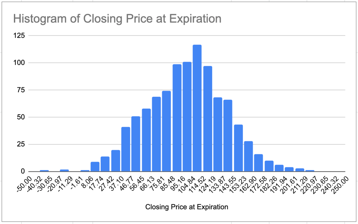
The results of the Monte-Carlo simulation are summarized at the left/middle side of the spreadsheet. We can see that the mean and standard deviation measured from the simulated trades are very close to the ones we used as input, which shows that our simulated trades were generated properly, and our sample size is large enough.
The win rates are reported for each leg. Since this is a call credit spread, a “WIN” for the seller is when both legs expire OTM. The leg 1 win rate tells us that this occurred 61.3% of the time in this simulation.
The leg 2 win rate is a little misleading here because it looks at the long call in a vacuum, as if it were traded on its own, not part of a spread. If it were bought on its own, the trader would want it to close ITM, hence this would be expected to happen 28.2% of the time according to the simulation results.
However, since this option is part of a spread, having it close ITM is considered a loss for the spread because whatever winnings it would generate would be wiped out by larger losses from the short leg. The reason it is reported here is because this template was designed for individual options as well as spreads, so we can just ignore it for this study.

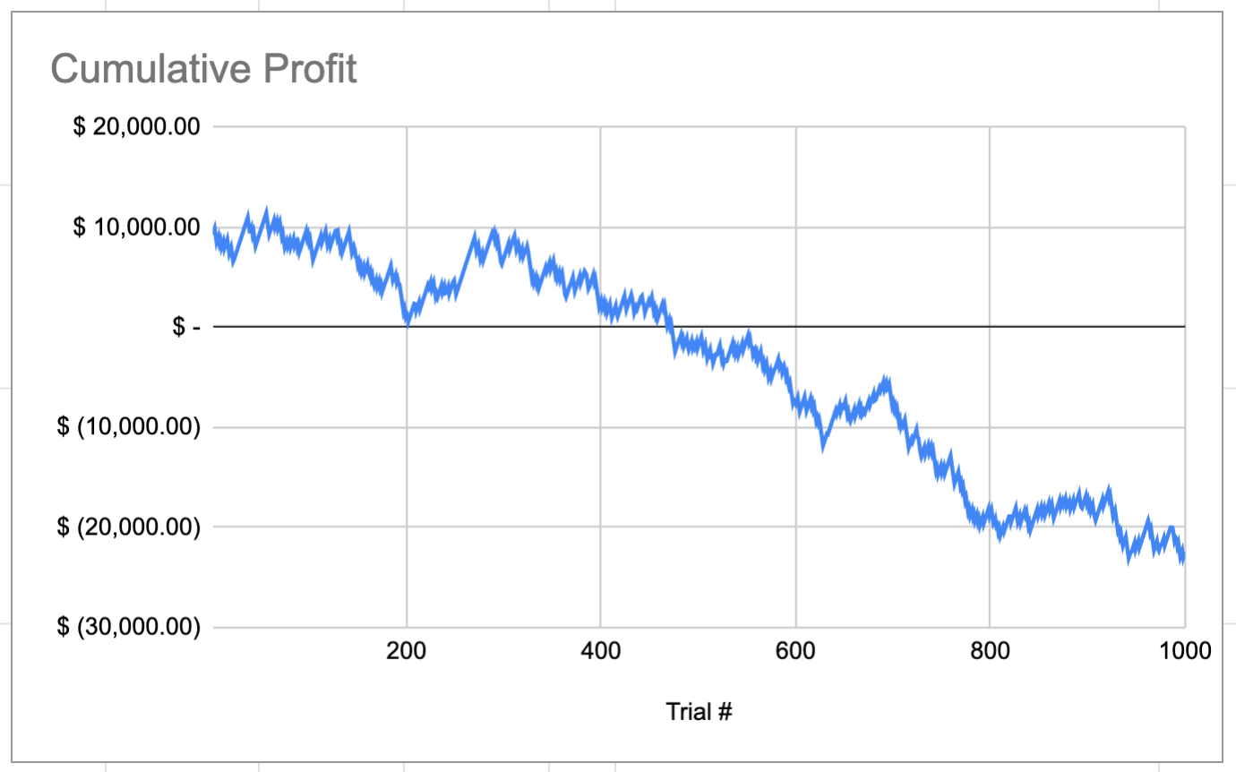
The results of this simulation show that the ending account balance is -$22.4k, for a total loss of $32.4k.
The following graphs show the distribution of simulated closing prices, as well as the cumulative account balance over the course of the one thousand simulated trades. Note that negative prices were allowed in this simulation to make the math easier, and although this is not realistic, they are not expected to affect the results very much because their probabilities of occurrence are extremely low, so there are only a few trades in the dataset with a negative closing price.
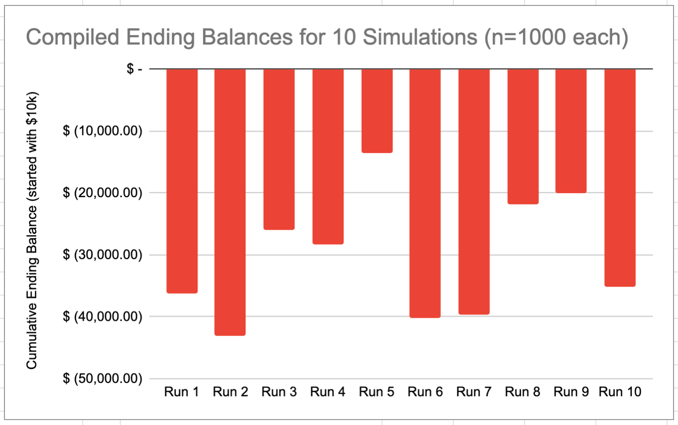
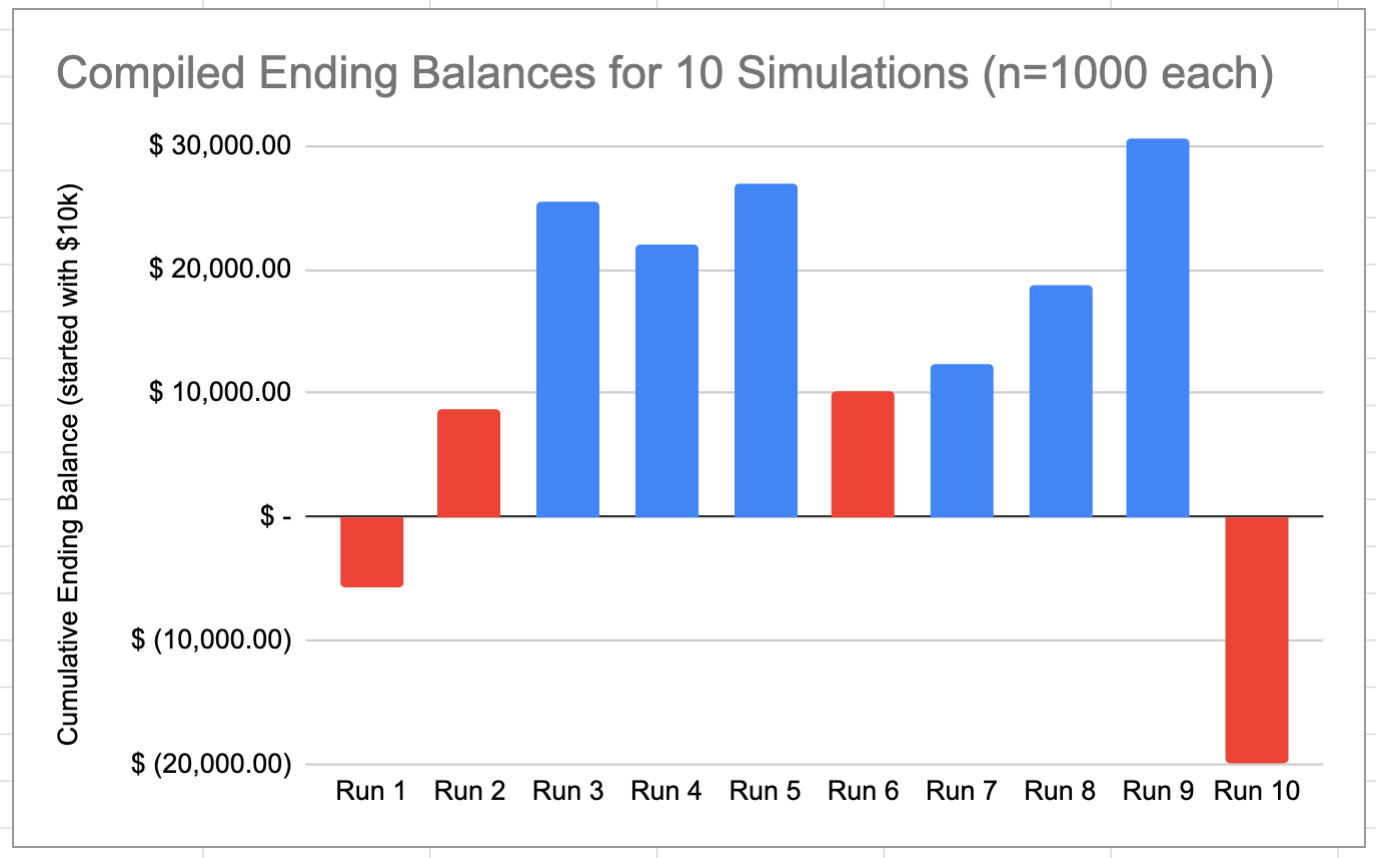
Obviously, these results are not good. Just to be sure they are consistent, we can re-run the simulation several more times and look at the ending balance for each run.
We can see that the results vary quite a bit, and all of them involve the trader losing all their money and going negative. This is a glaring indication that the expected value rule is not accurate. The actual premium required to not lose all your money in the long term is higher than what the expected value rule suggests.
We might ask, what would the input values need to be to make these results better? Specifically, we can increase the net premium until we consistently see the ending balance fall above the $10k we started with.
After a little experimentation, it seems like using a net premium of $3.50 results in a roughly 60/40 mix of ending balances above and below the initial $10k. Presumably the results will get better from here as the net premium increases. We could consider this the true break-even premium that would be required for the trade to be profitable.

There is still a lot of variation in the results between runs. This suggests that perhaps 1,000 trades per run is not enough, because running the simulation 10 times with 1,000 trades each is basically the same as running it once with 10,000 trades. Perhaps a larger overall sample size would make the results more consistent.
However, 1,000 trades is already ridiculous. If I need to make 1,000+ trades before I find out whether my strategy is profitable, then this is not something I would sign up for. This is the main reason I did this study in the first place – to avoid learning this the hard way.
Furthermore, it is not necessarily realistic to do this many trades in a reasonable amount of time even if you wanted to. Let’s say the spreads that provide the necessary premium to make the strategy viable are all 1-month term. There is a limit to how many of these trades the average retail trader could put on. Even if trades were cycled in and out each day, so that every month 30 trades were opened and 30 were closed, that would only be 30 trades per month. It would take 2.8 years to do 1,000 of those trades.
Not to mention, this would also be very capital intensive. Having 30 trades on at once, each with a MAX loss of $1,000, would require $30k in cash collateral. If this strategy is done safely with only a small percentage of the account, say 10%, this would require a $300k account. Perhaps this could work for an institutional trader, but not for the average retail trader.
I have not repeated this simulation with a variety of different stocks/ETFs at different strikes, expirations, spread widths, etc., so it is possible that the results could look better in a different scenario. Feel free to run your own simulations and see if a given trade is expected to be profitable in the long term.
One last thing I would like to look at is whether the minimum credit required to be profitable is actually possible to find in the market. After all, if the market doesn’t offer you the premium you need to make your trade profitable, then you’re out of luck.
Originally, we got a minimum required credit of $3.00 from the expected value table, but after running the Monte-Carlo simulation, that minimum credit seemed to be more like $3.50, so the accuracy of the expected value rule has already come into question, but we’ll put that aside for now.
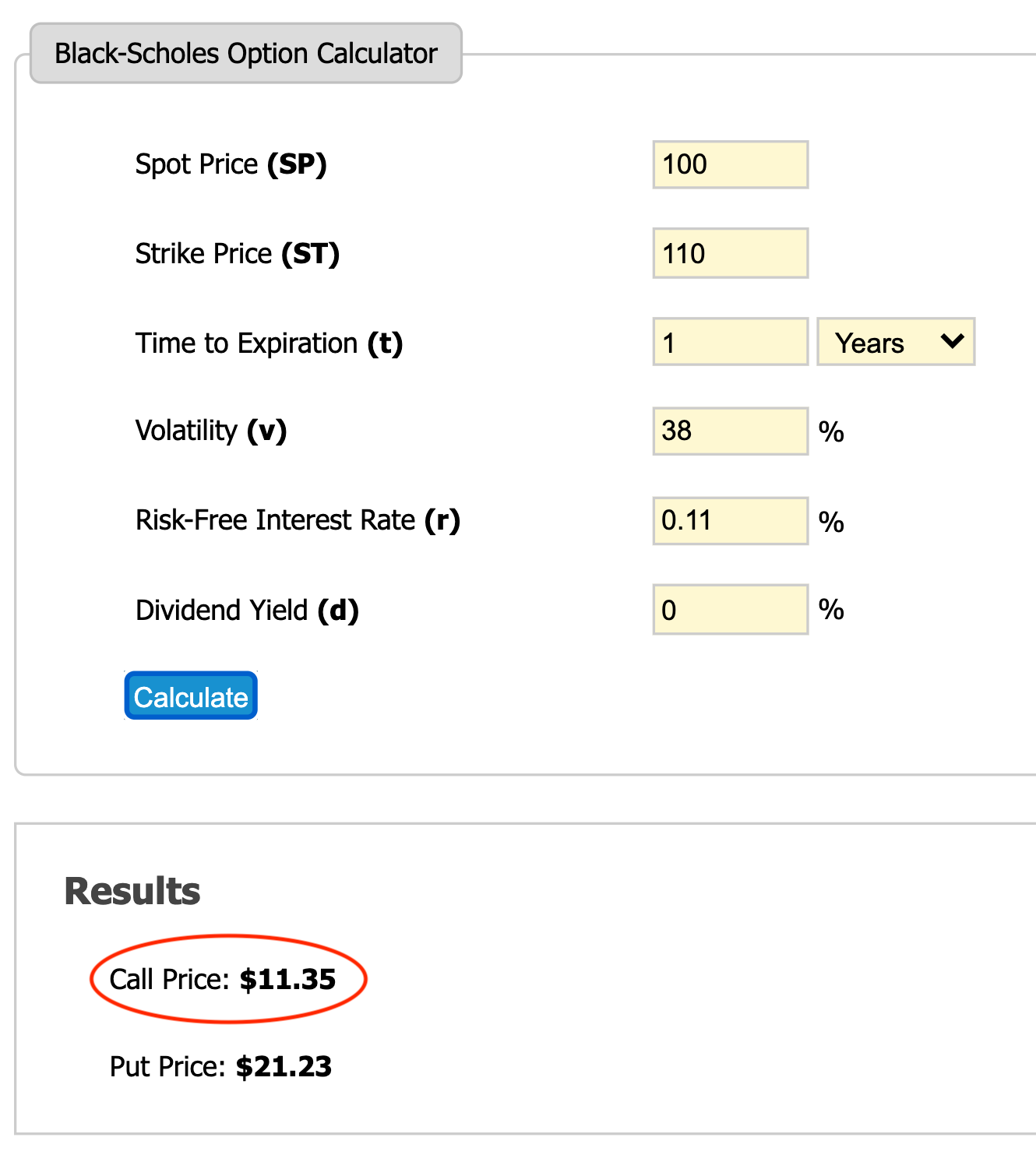
Let’s try to get more realistic option prices for our XYZ example. We can calculate the option price for each leg using this Black-Scholes calculator. Black-Scholes is the classic model for option pricing that can tell us the theoretical value of each of our options given the input parameters from our simulation.
Below are the Black-Scholes calculations for both legs of our example call credit spread. For the risk-free interest rate, we will use the current U.S. 3-month Treasury Bill interest rate, which is 0.11% as of November 9, 2020, per FRED. We will also assume that our hypothetical stock XYZ pays no dividends.
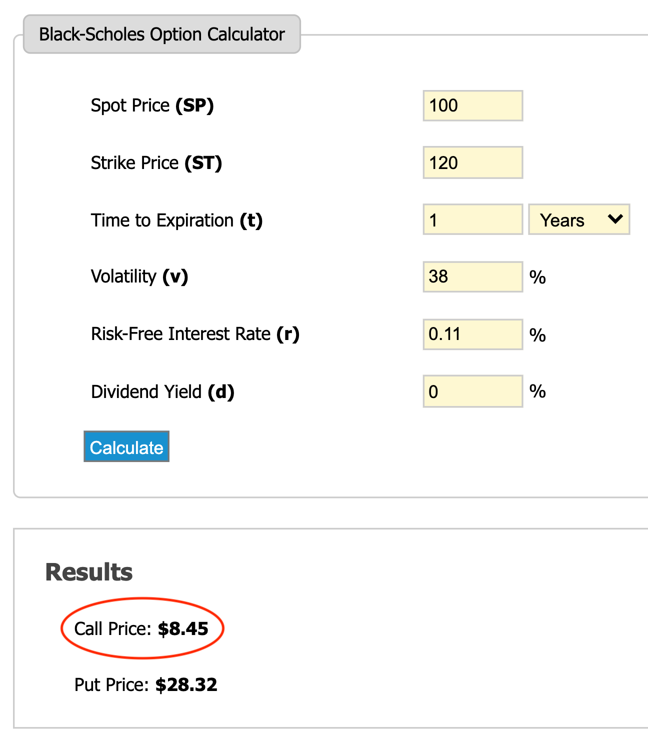
These prices result in a net premium of $2.90 for the spread. This is $0.10 below the $3.00 minimum recommended by the expected value table to break-even, and $0.60 below the $3.50 minimum derived from the Monte-Carlo results to achieve roughly 50/50 good and bad outcomes. This actual premium does not meet either of our standards, both of which are pretty low.
Below are the results for running the simulation 10 times using a net premium of $2.90.

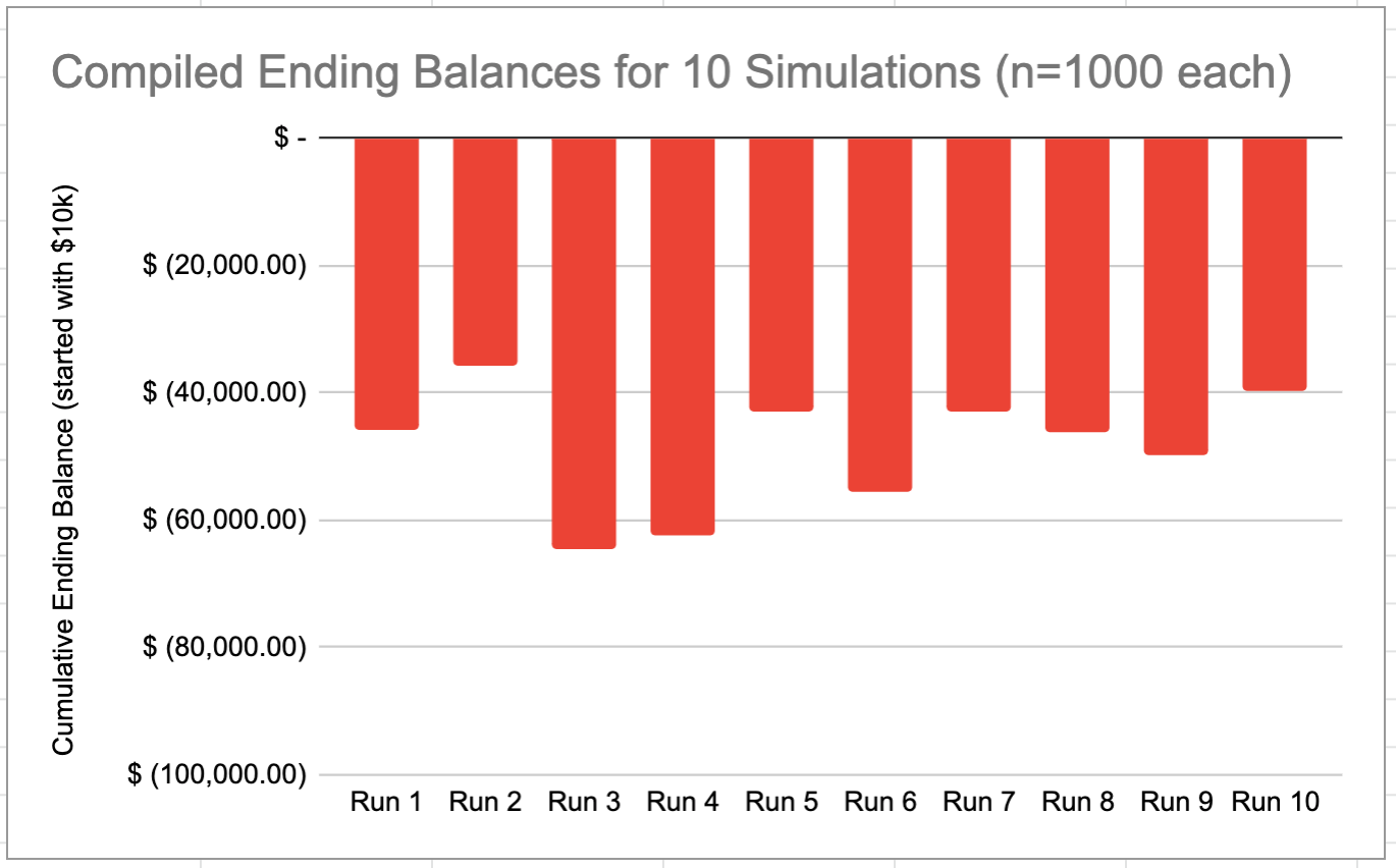
Unsurprisingly, these results are worse than those for the $3.00 premium. The ending account balance is between -$35k and -$65k in every case. These results are very concerning. If the market follows the Black-Scholes formula, this suggests it will be unlikely for us to find trades that meet our criteria for profitability.
It is certainly possible that the market is not most accurately represented by the Black-Scholes formula. One reason is the fact that Black-Scholes assumes European style options (which must be held until expiration), whereas I am trading in the U.S. where options can be bought and sold at any time during their life.
However, this study assumes European style options as well, so using Black-Scholes to determine the input option prices should accurately represent the trading strategy being studied.
Considering the reality that U.S. style options can be bought and sold at any time, it is an open question in my mind whether a trader in the U.S. can adjust their positions effectively enough over the option lifetimes to tilt the results in their favor. I am doubtful that this can be done reliably and consistently.
Summary
In summary, these simulation results suggest that the theory behind selling options to collect consistent premiums like an insurance company is not fully sound, at least in the form in which I have seen it evangelized. The market does not seem to offer premiums that are high enough for these types of trades to be viable in the long term.
The caveat is that no real options were used in this study. Now that the expected value rule and the Monte Carlo results have been established, I can more easily survey the market and see whether “good trades” actually exist because I know what I am looking for. I will keep my eyes open, and perhaps I will follow up with another post about this in the future, but I would encourage you to test the simulation with your own option data as well.
Thanks for reading! §